This project is part of a follow-up effort to my Mathematica Class Demonstrations project. While I do still enjoy using Mathematica since it's so quick and easy (and I hate doing algebra by hand), unfortunately most people don't have access to it, which significantly limits the potential audience for my previously-uploaded demonstrations. Aside from (and even with) Wolfram Demonstrations there isn't really a good way to make Mathematica files available online, so in late 2020 I started to look around for some alternatives.
I came across a partial solution in the January 2021 issue of SIAM News, which included an article about a recently-published interactive textbook made in the form of a Jupyter Notebook. I had heard about and briefly looked into Jupyter Notebooks previously while teaching myself Python, but they seemed hard so I stopped. I also wasn't aware that they had the potential to make interactive widgets similar to Mathematica's Manipulate function, but after seeing what they could do I set out to try to learn how to remake some of my old Mathematica projects using Jupyter Notebooks.
This is still a work in progress. Jupyter Notebooks are a huge pain to develop as compared to Mathematica demonstrations, and I certainly don't expect to be able to port all of my old projects over, but I expect to be adding more over the years alongside some other web app formats.
Jupyter Notebooks are primarily meant for sharing code which can be executed by a server, which makes them great for computable notebooks, but I wanted to try to keep the output as simple as possible so that the user wouldn't have to think about or even look at the source code while looking at the interactive widgets. Normally a service like Binder would display the notebook as a sequence of executable cells, so in order to simplify the presentation all of the links below are run through Voilà and rendered as standalone web apps.
In addition, unlike the original Mathematica projects I've made more of an effort here to work the interactive widgets into a full mini-lesson with all of the necessary explanatory text. Most of the projects below link to more than one notebook, including a full explanation as well as just the main interactive widget by itself.

Created 4/20/2021
Original Mathematica Demonstration
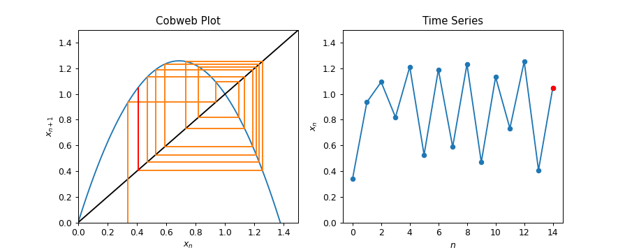
This demonstration gives a brief introduction to cobwebbing, a graphical technique for quickly approximating the general behavior of a discrete dynamical system. This is a useful technique in mathematical biology since many population growth models take the form of a difference equation. In particular, if the population in the next time step is given as a function \(f\) of the population in the current time step, then the cobweb plot can be used to estimate the sequence of population values over many time steps by drawing a zig-zagging line alternately between the \(y = f(x)\) curve and the \(y = x\) line. The complete demonstration includes an explanation for the motivation behind cobweb diagrams and the reasoning behind why they work, and goes through a few population models as examples. The standalone version includes only a pair of interactive widgets showing the process of drawing cobweb plots for two systems with adjustable parameters.
Tags: Chaos, Discrete Mathematics, Dynamical Systems, Mathematical Modeling, Pretty Pictures


Created 4/17/2021
Original Mathematica Demonstration
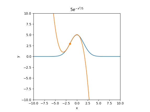
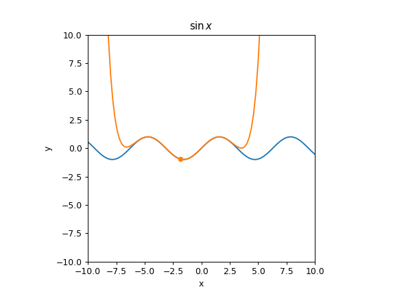
This demonstration shows how a Taylor series approximation of a given function changes as more terms are added to the series. The complete demonstration includes a mini-lesson showing how the Taylor series can be arrived at by building up a sequence of increasingly-complicated polynomial approximations, while the standalone widget includes only the final widget for manipulating the center and degree of the approximation for a variety of test functions. These can be used to show how well the approximations model the original function near or far from the center, and how adding more terms changes things.
Tags: Analysis, Calculus, Computational Mathematics